BCB420 - Computational System Biology
R - Basics
last modified 2022-12-29
Chapter 1 About
Original content for this book was created by Boris Steipe from Boris Steipe BCB420 wiki resources licensed under ![]() CC BY 4.0.
CC BY 4.0.
1.1 Attributions:
This book was created using The bookdown package and can be installed from CRAN or Github:
install.packages("bookdown")
# or the development version
# devtools::install_github("rstudio/bookdown")
Icons are from the “Very Basic. Android L Lollipop” set by Ivan Boyko licensed under CC BY 3.0.
#Installing R and RStudio {#r_install} (Notation; installing R and RStudio; packages; first experiments.)
1.2 Overview
###Abstract: This unit works through the installation of R and RStudio on your machine as well as through docker and introduces R’s packages of additional functions.
1.2.1 Objectives:
This unit will:
- guide you through first steps for installing R and R Studio on your own computer; and
- guide you through installing and using R and R Studio through docker; and
- introduce the concept of “packages” to extend R’s functionality;
1.2.2 Outcomes:
After working through this unit you:
- have a working installation of R and RStudio and know how to start RStudio;
- have a working knowledge of docker and how to use it with R and Rstudio.
- can find and install packages.
1.2.3 Deliverables:
Time management: Before you begin, estimate how long it will take you to complete this unit. Then, record in your course journal: the number of hours you estimated, the number of hours you worked on the unit, and the amount of time that passed between start and completion of this unit.
Journal: Document your progress in your Course Journal. Some tasks may ask you to include specific items in your journal. Don’t overlook these.
Insights: If you find something particularly noteworthy about this unit, make a note in your insights! page.
1.3 R
1.3.1 Introduction
The R statistics environment and programming language is an exceptionally well engineered, free (as in free speech) and free (as in free beer) platform for data manipulation and analysis. The number of functions that are included by default is large, there is a very large number of additional, community-generated analysis modules that can be simply imported from dedicated sites (e.g. the Bioconductor project for molecular biology data), or via the CRAN network, and whatever function is not available can be easily programmed. The ability to filter and manipulate data to prepare it for analysis is an absolute requirement in research-centric fields such as ours, where the strategies for analysis are constantly shifting and prepackaged solutions become obsolete almost faster than they can be developed. Besides numerical analysis, R has very powerful and flexible functions for plotting graphical output.
Note: you can’t learn a programming language in a single day.
Work through this material unit by unit, but when you are done, you need constant repetition to bring it into active memory. And make sure you understand every step. Taking shortcuts and/or cramming everything in a single, desperate effort is a waste of your time.
1.3.2 Before you begin: Notation and Formatting
In this tutorial, I use specific notation and formatting to mean different things:
- If you see footnotes1, click on the number to read more.
- This is normal text for explanations. It is written in a proportionally spaced font.
Code formatting is for code examples, file- and function names, directory paths etc. Code is written in a monospaced font2.
for (i in 1:10){
  #example code block
}- Bold emphasis and underlining are to mark words as particularly important.
- Examples of the right way to do something are highlighted green.
- Examples of the wrong way to do something are highlighted red.
1.3.3 Task - example
Tasks and exercises are described in boxes with a blue background. It is highly recommended that you do them. You won’t be graded on them but they are all content you can add to your journal. If you have problems, you must contact your instructor, or discuss the issue on the mailing list. Don’t simply continue. All material builds on previous material, and evaluation is cumulative.
These sections have information about issues I encounter more frequently. They are required reading when you need to troubleshoot problems but also give background information that may be useful to avoid problems in the first place.
1.3.4 “Metasyntactic variables”
When I use notation like <Year> in instructions, you type the year, the whole year and nothing but the year (e.g the four digits 2017). You never type the angle brackets! I use the angle brackets only to indicate that you should not type Year literally, but substitute the correct value. You might encounter this notation as <path>, <filename>, <firstname lastname> and similar. To repeat: if I specify
<your name>… and your name is Elcid Barrett, You type
Elcid Barrett… and not your name or <Elcid Barret> or similar. (Oh the troubles I’ve seen …)
The sample code on this page sometimes copies text from the console, and sometimes shows the actual commands only. The > character at the beginning of the line is always just R’s input prompt, it tells you that you can type something now - you never actually type > at the beginning of a line. If you read:
> getwd()you need to type:
getwd()If a line starts with [1] or similar, this is R’s output on the console.3
The # character marks the following text as a comment which is not executed by R. These are lines that you do not type. They are program output, or comments, not commands.
1.3.5 Characters
Different characters mean different things for computers, and it is important to call them by their right name.
- / ◁ this is a forward-slash. It leans forward in the reading direction.
- \ ◁ this is a backslash. It leans backward in the reading direction.
- ( ) ◁ these are parentheses.
- ◁ these are (square) brackets.
- < > ◁ these are angle brackets.
- { } ◁ these are (curly) braces.
- ” ◁ this, and only this is a quotation mark or double quote. All of these are not: “”„«» . They will break your code. Especially the first two are often automatically inserted by MSWord and hard to distinguish.Never, ever edit code in MS Word. Use R or RStudio. Actually, don’t use notepad or TextEdit either.
- ’ ◁ this, and only this is a single quote. All of these are not: ’’‚‹› . They will break your code. Especially the first two are often automatically inserted by MSWord and hard to distinguish.
MSWord is not useful as a code editor.
1.4 The environment
In this section we discuss how to download and install the software, how to configure an R session and how to work in the R environment.
There are many different ways you can use and setup R. By simply installing R you can use it directly but it is highly recommended that you also install and use RStudio which is an Integrate development environment (IDE) for R. You cannot just download RStudio and use it. It requires an installation of R.
You don’t need to install R and RStudio though. You can also use R and RStudio through docker. I highly recommend using docker instead
As with many open source projects, R is a constantly evolving language with regular updates. There is a major release once a year with patch releases through out the year. Often scripts and packages will work from one release to the next (ignoring pesky warnings that a package was compiled on a previous version of R is common) but there are exceptions. Some newer packages will only work on the latest version of R so sometimes the choice of upgrading or not using a new package might present themselves. Often, the amount of packages and work that is need to upgrade is not realized until the process has begun. This is where docker demonstrates it most valuable features. You can create a new instance based on the latest release of R and all your needed packages without having to change any of your current settings.
If you want you can skip over installing R and and Rstudio and go directly to install docker. There is no requirement to do both. I would recommend going straight to docker!
1.5 Task 1 - Install R
- Navigate to CRAN (the Comprehensive R Archive Network) and follow the link to Download R for your computer’s operating system. * You can also use one of the mirror sites, if CRAN is down - for example the mirror site at the University of Toronto. A choice of mirror sites is listed on the R-project homepage.
- Download a precompiled binary (or build) of the R framework to your computer and follow the instructions for installing it. Make sure that the program is the correct one for your version of your operating system.
- Launch R.
- Once you see that R is running correctly, you may quit the program for now.
I can’t install R.
- Make sure that the version you downloaded is the right one for your operating system.
- Also make sure that you have the necessary permissions on your computer to install new software.
1.6 Task 2 - Install RStudio
RStudio is a free IDE (Integrated Development Environment) for R. RStudio is a wrapper4 for R and as far as basic R is concerned, all the underlying functions are the same, only the user interface is different (and there are a few additional functions that are very useful e.g. for managing projects).
Here is a small list of differences between R and RStudio.
pros (some pretty significant ones actually):
- Integrated version control.
- Support for “projects” that package scripts and other assets.
- Syntax-aware code colouring.
- A consistent interface across all supported platforms. (Base R GUIs are not all the same for e.g. Mac OS X and Windows.)
- Code autocompletion in the script editor. (Depending on your point of view this can be a help or an annoyance. I used to hate it. After using it for a while I find it useful.)
- “Function signaturtes” (a list of named parameters) displayed when you hover over a function name.
- The ability to set breakpoints for debugging in the script editor.
- Support for knitr, and rmarkdown; also support for R notebooks … (This supports “literate programming” and is actually a big advance in software development)
- Support for R notebooks.
cons (all minor actually):
- The tiled interface uses more desktop space than the windows of the R GUI.
- There are sometimes (rarely) situations where R functions do not behave in exactly the same way in RStudio.
- The supported R version is not always immediately the most recent release.
- Navigate to the RStudio download Website.
- Find the right version of the RStudio Desktop installer for your computer, download it and install the software.
- Open RStudio.
-
Focus on the bottom left pane of the window, this is the “console”
pane.
- Type getwd().
- This prints out the path of the current working directory. Make a (mental) note where this is. We usually always need to change this “default directory” to a project directory.
1.7 Docker
Changing versions and environments are a continuing struggle with bioinformatics pipelines and computational pipelines in general. An analysis written and performed a year ago might not run or produce the same results when it is run today. Recording package and system versions or not updating certain packages rarely work in the long run.
One the best solutions to reproducibility issues is containing your workflow or pipeline in its own coding environment where everything from the operating system, programs and packages are defined and can be built from a set of given instructions. There are many systems that offer this type of control including:
“A container is a standard unit of software that packages up code and all its dependencies so the application runs quickly and reliably from one computing environment to another.” (“What Is a Container?” n.d.)
Why are containers great for Bioiformatics?
- allows you to create environments to run bioinformatis pipelines.
- create a consistent environment to use for your pipelines.
- test modifications to the pipeline without disrupting your current set up.
- Coming back to an analysis years later and there is no need to install older versions of packages or programming languages. Simply create a container and re-run.
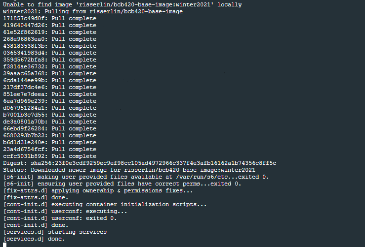
All assignments for this course are expected to compile and run. We will be using the bcb420-base-image:winter2023 docker image to run all or your submitted notebooks. If your notebook runs with no errors and renders your html notebook you will recieve full marks for compilation. It is recommended that you do all your work and assignments using this docker image.
1.7.1 What is docker?
- Docker is a container platform, similar to a virtual machine but better.
- We can run multiple containers on our docker server. A container is an instance of an image. The image is built based on a set of instructions but consists of an operating system, installed programs and packages. (When backing up your computer you might taken an image of it and restored your machine from this image. It the same concept but the image is built based on a set of elementary commands found in your Dockerfile.) - for overview see here
- Often images are built off of previous images with specific additions you need for you pipeline. (For example, for this course we use a base image supplied by bioconductorrelease 3.11 and comes by default with basic Bioconductor packages but it builds on the base R-docker images called rocker.)
1.8 Docker - Basic term definition
1.8.1 Container
- An instance of an image.
- the self-contained running system.
- There can be multiple containers derived from the same image.
1.8.2 Image
- An image contains the blueprint of a container.
- In docker, the image is built from a Dockerfile
1.8.3 Docker Volumes
- Anything written on a container will be erased when the container is erased ( or crashes) but anything written on a filesystem that is separate from the contain will persist even after a container is turned off.
- A volume is a way to assocaited data with a container that will persist even after the container. * maps a drive on the host system to a drive on the container.
- In the above docker run command (that creates our container) the statement:
-v ${PWD}:/home/rstudio/projects- maps the directory ${PWD} to the directory /home/rstudio/projects on the container. Anything saved in /home/rstudio/projects will actually be saved in ${PWD}
- An example:
- I use the following commmand to create my docker container:
docker run -e PASSWORD=changeit --rm \
  -v /Users/risserlin/bcb420_code:/home/rstudio/projects \
  -p 8787:8787 \
risserlin/bcb420-base-image:winter2023- I create a notebook called task3_bcb420.Rmd and save it in /home/rstudio/projects.
Note: Do not save it in /home/rstudio/ which is the default directory RStudio will start in
- On my host computer, if I go to /Users/risserlin/bcb420_code I will find the file task3_bcb420.Rmd
1.9 Task 3 - Install Docker
- Download and install docker desktop.
- Follow slightly different instructions for Windows or MacOS/Linux
1.9.1 Windows
- it might prompt you to install additional updates (for example - https://docs.Microsoft.com/en-us/windows/wsl/install-win10#step-4---download-the-linux-kernel-update-package) and require multiple restarts of your system or docker.
- launch docker desktop app.
- Open windows Power shell
- navigate to directory on your system where you plan on keeping all your code. For example: C:\USERS\risserlin\bcb420_code
- Run the following command: (the only difference with the windows command is the way the current directory is written. ${PWD} instead of "$(pwd)")
docker run -e PASSWORD=changeit --rm \
  -v ${PWD}:/home/rstudio/projects -p 8787:8787 \
  risserlin/bcb420-base-image:winter2023
- Windows defender firewall might pop up with warning. Click on Allow access.
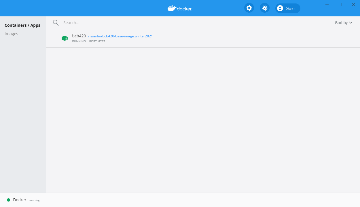
- In docker desktop you see all containers you are running and easily manage them.
1.9.2 MacOS / Linux
- Open Terminal
- navigate to directory on your system where you plan on keeping all your code. For example: /Users/risserlin/bcb420_code
- Run the following command: (the only difference with the windows command is the way the current directory is written. ${PWD} instead of "$(pwd)")
docker run -e PASSWORD=changeit --rm \
  -v "$(pwd)":/home/rstudio/projects -p 8787:8787 \
  risserlin/bcb420-base-image:winter2023
1.10 Task 4 - Create your first notebook using Docker
1.10.1 Start coding!
- Open a web browser to localhost:8787
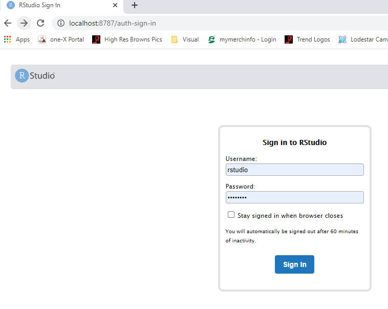
- enter username: rstudio
- enter password: changeit
- changing the parameter -e PASSWORD=changeit in the above docker command will change the password you need to specify
When you go to localhost:8787 all you get is:
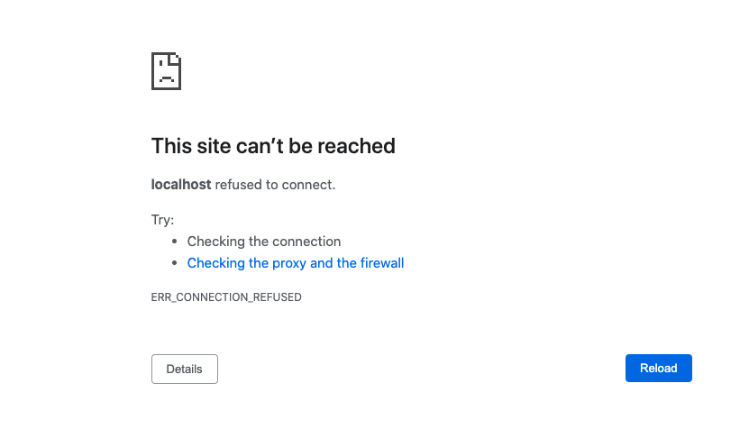
- Make sure your docker container is running. (If you rebooted your machine you will need to restart the container on reboot.)
- Make sure you got the right port.
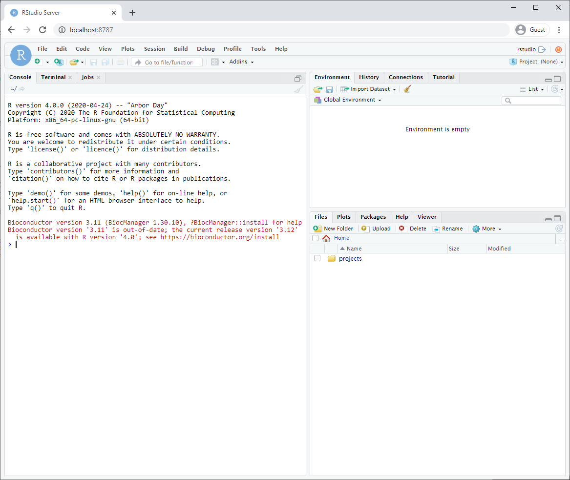
After logging in, you will see an Rstudio window just like when you install it directly on your computer. This RStudio will be running in your docker container and will be a completely separate instance from the one you have installed on your machine (with a different set of packages and potentially versions installed).
Make sure that you have mapped a volume on your computer to a volume in your container so that files you create are also saved on your computer. That way, turning off or deleting your container or image will not effect your files.
- The parameter -v ${PWD}:/home/rstudio/projects maps your current directory (i.e. the directory you are in when launching the container) to the directory /home/rstudio/projects on your container.
- You do not need to use the ${PWD} convention. You can also specify the exact path of the directory you want to map to your container.
- Make sure to save all your scripts and notebooks in the projects directory.
- Create your first notebook in your docker Rstudio.
- Save it.
- Find your newly created file on your computer.
1.11 Packages
R has many powerful functions built in, but one of it’s greatest features is that it is easily extensible. Extensions have been written by legions of scientists for many years, most commonly in the R programming language itself, and made available through CRAN–The Comprehensive R Archive Network or through the Bioconductor project.
A package is a collection of code, documentation and (often) sample data. * To use packages, you need to install the package (once). * You can then use all of the package’s functions by prefixing them with the package name and a double colon (eg. package::function()); that’s the preferred way.
seqinr::bma(c("c","c","a"))- Or you can load all of the package’s functions with a library(package) command, and then use the functions without a prefix. That’s less typing, but it’s also less explicit and you may end up constantly wondering where exactly a particular function came from. In the teaching code for this course, I use the package::function() idiom wherever reasonable.
library(seqinr)
1.12 Task 5 - Experiment with RStudio and packages
- Navigate to http://cran.r-project.org/web/packages/ and read the page.
- Navigate to http://cran.r-project.org/web/views/ (the curated CRAN task-views).
- Follow the link to Genetics and read the synopsis of available packages. The library sequinr sounds useful, but check first whether it has been installed.
- Follow the exercise below
1.12.1 Exercise
In your RStudio window:
create a new notebook.
go though each of the commands below and add them to your notebook.
write your observation for each of commands in the notebook.
Add this new notebook to your github repo and link to it in your journal.
library() opens a window that lists the packages that are installed on your computer;
library()- search() - shows which ones are currently loaded.
search()## [1] ".GlobalEnv" "tools:rstudio" "package:stats"
## [4] "package:graphics" "package:grDevices" "package:utils"
## [7] "package:datasets" "package:methods" "Autoloads"
## [10] "package:base"- In the Packages tab of the lower-right pane in RStudio, confirm that seqinr is not yet installed.
- Follow the link to seqinr to see what standard information is available with a package. Then follow the link to the Reference manual to access the documentation pdf. This is also sometimes referred to as a “vignette” and contains usage hints and sample code.
- Read the help for vignette. Note that there is a command to extract R sample code from a vignette, to experiment with it.
?vignette- Install seqinr from the closest CRAN mirror and load it for this session. Explore some functions.
# to get help on using install.packages
?install.packages

# Note: the parameter is a quoted string!
install.packages("seqinr",repos="https://cran.rstudio.com/")
## Installing package into '/usr/local/lib/R/site-library'
## (as 'lib' is unspecified)## also installing the dependencies 'pixmap', 'ade4', 'segmented'- this will launch a new window with the seqinr package info
library(help="seqinr") - list all the functions available in the seqinr package.
#Note: the file must be attached in order for the below function to work
library(seqinr)
ls("package:seqinr")## [1] "a" "aaa"
## [3] "AAstat" "acnucclose"
## [5] "acnucopen" "al2bp"
## [7] "alllistranks" "alr"
## [9] "amb" "as.alignment"
## [11] "as.matrix.alignment" "as.SeqAcnucWeb"
## [13] "as.SeqFastaAA" "as.SeqFastadna"
## [15] "as.SeqFrag" "autosocket"
## [17] "baselineabif" "bma"
## [19] "c2s" "cai"
## [21] "cfl" "choosebank"
## [23] "circle" "clfcd"
## [25] "clientid" "closebank"
## [27] "col2alpha" "comp"
## [29] "computePI" "con"
## [31] "consensus" "count"
## [33] "countfreelists" "countsubseqs"
## [35] "crelistfromclientdata" "css"
## [37] "dia.bactgensize" "dia.db.growth"
## [39] "dist.alignment" "dotchart.uco"
## [41] "dotPlot" "draw.oriloc"
## [43] "draw.rearranged.oriloc" "draw.recstat"
## [45] "exseq" "extract.breakpoints"
## [47] "extractseqs" "fastacc"
## [49] "gb2fasta" "gbk2g2"
## [51] "gbk2g2.euk" "GC"
## [53] "GC1" "GC2"
## [55] "GC3" "GCpos"
## [57] "get.db.growth" "getAnnot"
## [59] "getAnnot.default" "getAnnot.list"
## [61] "getAnnot.logical" "getAnnot.qaw"
## [63] "getAnnot.SeqAcnucWeb" "getAnnot.SeqFastaAA"
## [65] "getAnnot.SeqFastadna" "getAttributsocket"
## [67] "getFrag" "getFrag.character"
## [69] "getFrag.default" "getFrag.list"
## [71] "getFrag.logical" "getFrag.qaw"
## [73] "getFrag.SeqAcnucWeb" "getFrag.SeqFastaAA"
## [75] "getFrag.SeqFastadna" "getFrag.SeqFrag"
## [77] "getKeyword" "getKeyword.default"
## [79] "getKeyword.list" "getKeyword.logical"
## [81] "getKeyword.qaw" "getKeyword.SeqAcnucWeb"
## [83] "getLength" "getLength.character"
## [85] "getLength.default" "getLength.list"
## [87] "getLength.logical" "getLength.qaw"
## [89] "getLength.SeqAcnucWeb" "getLength.SeqFastaAA"
## [91] "getLength.SeqFastadna" "getLength.SeqFrag"
## [93] "getlistrank" "getliststate"
## [95] "getLocation" "getLocation.default"
## [97] "getLocation.list" "getLocation.logical"
## [99] "getLocation.qaw" "getLocation.SeqAcnucWeb"
## [101] "getName" "getName.default"
## [103] "getName.list" "getName.logical"
## [105] "getName.qaw" "getName.SeqAcnucWeb"
## [107] "getName.SeqFastaAA" "getName.SeqFastadna"
## [109] "getName.SeqFrag" "getNumber.socket"
## [111] "getSequence" "getSequence.character"
## [113] "getSequence.default" "getSequence.list"
## [115] "getSequence.logical" "getSequence.qaw"
## [117] "getSequence.SeqAcnucWeb" "getSequence.SeqFastaAA"
## [119] "getSequence.SeqFastadna" "getSequence.SeqFrag"
## [121] "getTrans" "getTrans.character"
## [123] "getTrans.default" "getTrans.list"
## [125] "getTrans.logical" "getTrans.qaw"
## [127] "getTrans.SeqAcnucWeb" "getTrans.SeqFastadna"
## [129] "getTrans.SeqFrag" "getType"
## [131] "gfrag" "ghelp"
## [133] "gln" "glr"
## [135] "gls" "is.SeqAcnucWeb"
## [137] "is.SeqFastaAA" "is.SeqFastadna"
## [139] "is.SeqFrag" "isenum"
## [141] "isn" "kaks"
## [143] "kdb" "knowndbs"
## [145] "lseqinr" "modifylist"
## [147] "move" "mv"
## [149] "n2s" "oriloc"
## [151] "parser.socket" "peakabif"
## [153] "permutation" "pga"
## [155] "plot.SeqAcnucWeb" "plotabif"
## [157] "plotladder" "plotPanels"
## [159] "pmw" "prepgetannots"
## [161] "prettyseq" "print.qaw"
## [163] "print.SeqAcnucWeb" "query"
## [165] "quitacnuc" "read.abif"
## [167] "read.alignment" "read.fasta"
## [169] "readBins" "readfirstrec"
## [171] "readPanels" "readsmj"
## [173] "rearranged.oriloc" "recstat"
## [175] "residuecount" "reverse.align"
## [177] "rho" "rot13"
## [179] "s2c" "s2n"
## [181] "savelist" "SEQINR.UTIL"
## [183] "setlistname" "splitseq"
## [185] "stresc" "stutterabif"
## [187] "summary.SeqFastaAA" "summary.SeqFastadna"
## [189] "swap" "syncodons"
## [191] "synsequence" "tablecode"
## [193] "test.co.recstat" "test.li.recstat"
## [195] "translate" "trimSpace"
## [197] "uco" "ucoweight"
## [199] "where.is.this.acc" "words"
## [201] "words.pos" "write.fasta"
## [203] "zscore"- In Rstudio this will open the method description for the method a in the Help pane.
?seqinr::a - Run the fiction to see the output
seqinr::a("Tyr")## [1] "Y"- What does function below do? enter your results in your journal
seqinr::words(3, c("A", "G", "C", "U"))The installation fails.
- You might see an error message such as this:
Warning message:
package ‘XYZ’ is not available (for R version
3.2.2)
-
This can mean several things:
- The package is not available on CRAN. Try Bioconductor instead or Google for the name to find it.
- The package requires a newer version of R than the one you have. Upgrade, or see if a legacy version exists.
- A comprehensive set of reasons and their resolution is here on stackoverflow.
-
We have seen the following on Windows systems when typing library(help=“seqinr”) Error in formatDL(nm, txt, indent = max(nchar(nm, “w”)) + 3) :
incorrect values of ‘indent’ and ‘width’
- Anecdotally this was due to a previous installation problem with a mixup of 32-bit and 64-bit R versions, although another student told us that the problem simply went away when trying the command again. Whatever: Make sure you have the right R version installed for your operating system. Uninstall and reinstall when in doubt. Conflicting libraries can be the source of strange misbehaviour.
The fact that these methods work, shows that the package has been downloaded, installed, its functions are now available with the package name prefix and any datasets it contains can be loaded. Just like many other packages, seqinr comes with a number of datafiles. Try:
- What does this function do?
?data- What is an example of data that is available for the seqinr package?
data(package="seqinr") # list the available data- load ‘’aaindex’’. Describe this data. See here for more information.
data(aaindex, package="seqinr") - what is this?
?aaindex - two of the indices …
aaindex$FASG890101 ## $H
## [1] "FASG890101"
##
## $D
## [1] "Hydrophobicity index (Fasman, 1989)"
##
## $R
## [1] ""
##
## $A
## [1] "Fasman, G.D."
##
## $T
## [1] "Prediction of Protein Structure and the Principles of Protein Conformation"
##
## $J
## [1] "Plenum, New York 1989, page 457, Table XVII"
##
## $C
## [1] "MIYS990105 0.959 MIYS990103 0.957 MEIH800102 0.951MIYS990104 0.949 RACS770102 0.935 GUYH850101 0.934MIYS990102 0.929 MIYS990101 0.926 MEIH800101 0.919KRIW790101 0.914 GUYH850102 0.909 VINM940101 0.904KRIW790102 0.882 GUYH850104 0.872 RACS770101 0.872GRAR740102 0.872 CORJ870108 0.872 KARP850102 0.871OOBM770103 0.869 VINM940103 0.868 OOBM770101 0.868KRIW710101 0.865 KIDA850101 0.861 GUYH850103 0.860PUNT030102 0.853 PUNT030101 0.845 FUKS010104 0.844RACS770103 0.842 ROSM880102 0.839 JANJ780103 0.838VINM940102 0.836 PARJ860101 0.825 KUHL950101 0.821JANJ780101 0.813 FUKS010103 0.812 GUOD860101 -0.801DESM900101 -0.808 CORJ870105 -0.821 ROSM880105 -0.822PONP800106 -0.823 NADH010101 -0.838 CORJ870106 -0.841KYTJ820101 -0.844 CIDH920103 -0.846 CHOC760103 -0.849BASU050101 -0.856 JURD980101 -0.857 PLIV810101 -0.858BAEK050101 -0.859 CIDH920105 -0.860 ROBB790101 -0.860EISD860103 -0.863 CORJ870104 -0.865 CORJ870107 -0.871JANJ790102 -0.875 CORJ870103 -0.876 NADH010105 -0.877DESM900102 -0.879 BASU050102 -0.881 JANJ790101 -0.885CIDH920104 -0.903 JANJ780102 -0.903 MANP780101 -0.904PONP930101 -0.907 ZHOH040103 -0.910 FAUJ830101 -0.911PONP800108 -0.913 BASU050103 -0.915 CORJ870101 -0.921NISK800101 -0.923 MEIH800103 -0.924 CASG920101 -0.924WERD780101 -0.926 BIOV880102 -0.928 NADH010102 -0.929PONP800101 -0.932 PONP800103 -0.936 MIYS850101 -0.938PONP800102 -0.944 NADH010104 -0.944 NADH010103 -0.945NISK860101 -0.949 ROSG850102 -0.976 RADA880108 -0.977BIOV880101 -0.982"
##
## $I
## Ala Arg Asn Asp Cys Gln Glu Gly His Ile Leu Lys
## -0.21 2.11 0.96 1.36 -6.04 1.52 2.30 0.00 -1.23 -4.81 -4.68 3.88
## Met Phe Pro Ser Thr Trp Tyr Val
## -3.66 -4.65 0.75 1.74 0.78 -3.32 -1.01 -3.50aaindex$PONJ960101 ## $H
## [1] "PONJ960101"
##
## $D
## [1] "Average volumes of residues (Pontius et al., 1996)"
##
## $R
## [1] "PMID: 8950272"
##
## $A
## [1] "Pontius, J., Richelle, J. and Wodak, S.J."
##
## $T
## [1] "Deviations from standard atomic volumes as a quality measure for protein crystal structures"
##
## $J
## [1] "J. Mol. Biol 264, 121-136 (1996) (Disulfide bonded cysteine, 102.4)"
##
## $C
## [1] "HARY940101 0.989 CHOC750101 0.966 FAUJ880103 0.963TSAJ990102 0.962 CHOC760101 0.961 TSAJ990101 0.960BIGC670101 0.950 GOLD730102 0.947 FASG760101 0.945KRIW790103 0.943 CHAM820101 0.938 GRAR740103 0.937LEVM760102 0.930 LEVM760105 0.928 CHAM830106 0.917FAUJ880106 0.913 DAWD720101 0.873 ROSG850101 0.862RADA880106 0.860 LEVM760107 0.827 ZHOH040102 0.823RADA880103 -0.873"
##
## $I
## Ala Arg Asn Asp Cys Gln Glu Gly His Ile Leu Lys
## 91.5 196.1 138.3 135.2 114.4 156.4 154.6 67.5 163.2 162.6 163.4 162.5
## Met Phe Pro Ser Thr Trp Tyr Val
## 165.9 198.8 123.4 102.0 126.0 209.8 237.2 138.4- Let’s use the data:
- plot amino acid single-letter codes by hydrophobicity and volume.
- The values come from the dataset.
- Copy and paste the commands.
plot(aaindex$FASG890101$I,
aaindex$PONJ960101$I,
xlab="hydrophobicity", ylab="volume", type="n")
text(aaindex$FASG890101$I,
aaindex$PONJ960101$I,
labels=a(names(aaindex$FASG890101$I)))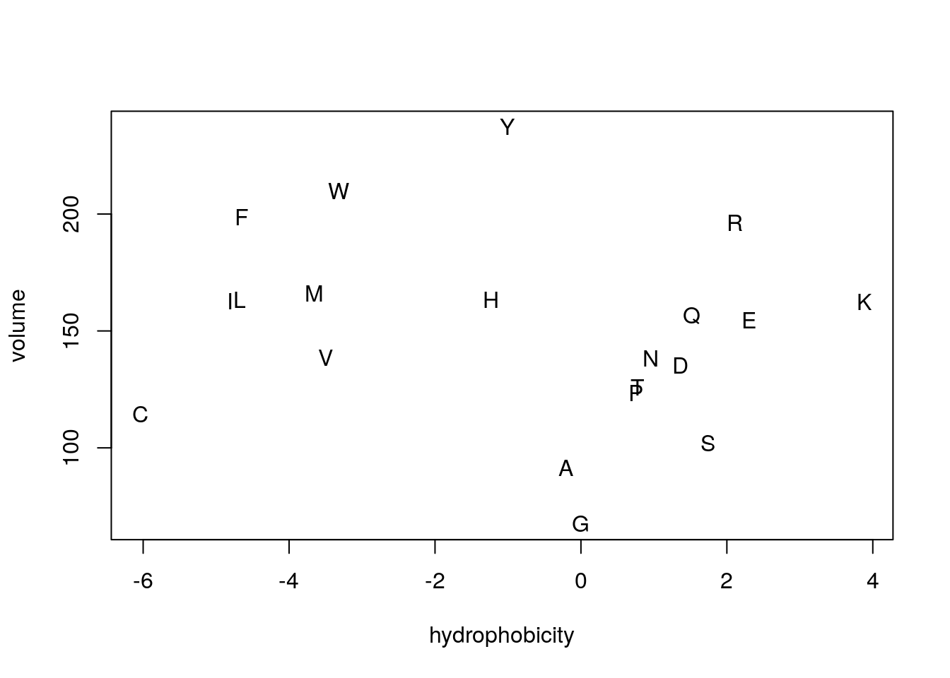
- Now, just for fun, let’s use seqinr package functions to download a sequence and calculate some statistics (however, not to digress too far, without further explanation at this point).
- Copy the code below and paste it into the R-console.
seqinr::choosebank("swissprot")
mySeq <- seqinr::query("mySeq", "N=MBP1_YEAST")
mbp1 <- seqinr::getSequence(mySeq)
seqinr::closebank()
x <- seqinr::AAstat(mbp1[[1]])
barplot(sort(x$Compo), cex.names = 0.6)We could have “loaded” the package with library(), and then used the functions without prefix. Less typing, but also less explicit.
library(seqinr)
choosebank("swissprot")
mySeq <- query("mySeq", "N=MBP1_YEAST")
mbp1 <- getSequence(mySeq)
closebank()
x <- AAstat(mbp1[[1]])
barplot(sort(x$Compo), cex.names = 0.6)In general we will be using the idiom with the package prefix throughout the course.
The function requireNamespace() is useful because it does not produce an error when a package has not been installed. It simply returns TRUE if successful or FALSE if not. Therefore one can use the following code idiom in R scripts to avoid downloading the package every time the script is called.
if (! requireNamespace("seqinr", quietly=TRUE)) {
install.packages("seqinr")
}You can get package information with the following commands:
library(help = seqinr) # basic informationbrowseVignettes("seqinr") # available vignettes## No vignettes found by browseVignettes("seqinr")data(package = "seqinr") # available datasets- Note that install.packages() takes a (quoted) string as its argument, but library() takes a variable name (without quotes). New users usually get this wrong :-)
- Note that the Bioconductor project has its own installation system, the Biocmanager::install() function. It is explained here.
- Note, just to mention it at this point: to install packages that are not on CRAN or Bioconductor, you need the devtools package.
1.12.2 Finding packages
One of the challenges of working with R is the overabundance of options. CRAN has over 10,000 packages and Bioconductor has over 1,300 more. How can you find ones that are useful to your work? There’s actually a package to help you do that, the sos package on CRAN. Try this:
if (! requireNamespace("sos", quietly=TRUE)) {
install.packages("sos")
}
library(help = sos) # basic information
browseVignettes("sos") # available vignettes
sos::findFn("moving average")Or:
- Read a CRAN Task View for your area of interest
- or the Bioconductor Views;
- Search on “Metacran” (“regex” example here”) …
- or “MRAN” (“regex” example here”, not that the results are not identical);
- and, as always, Google.
1.12.3 Self-evaluation
- Question 1 - What is the purpose of this code?
if (! requireNamespace("seqinr", quietly = TRUE)) {
install.packages("seqinr")
}Why not just use: install.packages(“seqinr”)
Answer: This code idiom is useful in scripts, to ensure a package is installed before we try to use its functions. If we would simply use install.packages(“seqinr”), the package would be downloaded from CRAN every time the script is run. That would make our script slow, and require available internet access for the script to run.
In the code above, the package is downloaded only when requireNamespace() returns FALSE, which presumably means the package has not yet been downloaded.
1.12.4 Further reading, links and resources
- Wikipedia article on the R statistics environment and programming language
- The R project homepage
- The R Studio IDE
- CRAN–The Comprehensive R Archive Network
- The Bioconductor project homepage
- R bloggers
- Package finding strategies (Revolutions Analytics Blog)
- Intro to R packages (at DataCamp).
- “The Impressive Growth of R” (Stackoverflow Data Analytics Team Blog)
- Ten simple rules for biologists learning to program - Carey and Papin advise novice biologist programmers how to begin. Much of this paper resonates well with our Introduction to R learning units. Good context for a beginning, to get a sense of where we are going with this.
If in doubt, ask!
If anything about this learning unit is not clear to you, do not proceed blindly but ask for clarification. Post your question on the course mailing list: others are likely to have similar problems. Or send an email to your instructor.
Author: Boris Steipe boris.steipe@utoronto.ca
Created: 2017-08-05
Modified: 2019-01-07
Version: 1.1
Version history:
1.1 Change from require() to requireNamespace() and use
1.02 Maintenance
1.0.1 Removed mention of Sweave - obsolete, and broken link. Added mention of “literate programming”.
1.0 Completed to first live version
0.1 Material collected from previous tutorial
1.12.5 Updated Revision history
## Installing package into '/usr/local/lib/R/site-library'
## (as 'lib' is unspecified)| Revision | Author | Date | Message |
|---|---|---|---|
| 5152496 | Ruth Isserlin | 2019-12-25 | Fixed issue with task numbering because of a remove all elements call in the 2nd chapter |
| fab47ae | Ruth Isserlin | 2019-12-24 | initial check in of R basics book |
1.13 Overview
###Abstract: This unit discusses the setup of a working session with RStudio.
1.13.1 Objectives:
This unit will:
- introduce R projects;
- start working with git version control via RStudio;
- discuss the history mechanism and why not to use it;
- mention .Rprofile to customize startup behaviour; and
- teach you to define the Working Directory of an R session.
1.13.2 Outcomes:
After working through this unit you:
- have verified that you can install R projects from GitHub;
- know what the .Rprofile file is for;
- can get and set the path of the current Working Directory.
1.13.3 Deliverables:
Time management: Before you begin, estimate how long it will take you to complete this unit. Then, record in your course journal: the number of hours you estimated, the number of hours you worked on the unit, and the amount of time that passed between start and completion of this unit.
Journal: Document your progress in your Course Journal. Some tasks may ask you to include specific items in your journal. Don’t overlook these.
Insights: If you find something particularly noteworthy about this unit, make a note in your insights! page.
1.14 Your Course Folder
Your Course Folder should already exist.
Take note! When you write a Windows paths in an R command, you have to use the “wrong” forward slash to separte directories and files. R will translate these “Unix-style”” paths into Windows-style paths automatically when it negotiates with the operating system. But the backslash is interpreted as an “escape” character that gives the character the follows it a special meaning.5
Folder name and path examples
/Users/Pierette/Documents/BCB420 ◁ Looking good on a Mac.
C:\Users\Pulcinella\Documents\CBW ◁ Looking good on a Windows computer.
“C:/Users/Pulcinella/Documents/CBW” ◁ Looking good inside R on a Windows computer (note the quotation marks!).
C:\Users\Pantalone\Documents\BCH1441 (2017) ◁ Wrong. No special characters please.
/Users/Brighella/Documents/UofT Stuffz/Courses/more/Comp Sys biol. course ◁ Wrong. Please read instructions more carefully.
C:\Users\Tartaglia\Documents\KUWTK\<Coursecode> ◁ I can’t even …
1.15 “Projects”
We will make extensive use of “projects” in class. Read more about projects in RStudio here.
1.16 Git Version control
We will also make extensive use of version control. In fact, we will now load a project via Git version control from its free, public repository on GitHub.
1.17 Task 6 - Git
- Read more about Version Control in RStudio here.
- Follow the instructions to install git on your computer.
Then do the following:
- open RStudio
- Select File → NewProject…
- Click on Version Control
- Click on Git
- Enter https://github.com/hyginn/R_Exercise-BasicSetup as the Repository URL.
-
Type a
character, the Project directory name field should then autofill to read R_Exercise-BasicSetup - Click on Browse… to find your Course Folder. (The one that you have already created). (If you are using docker make sure the directory you choose is in the projectes directory so it gets stored in your mapped volume on your machine)
- Click Open.
- Click Create Project; the project files should be downloaded and the console should prompt you to type init() to begin.
- Type init() into the console pane.
- An R script should load.
- Explore the script and follow its instructions.
-
I get an error message: “Git not found”. * The simplest reason is that you may have had RStudio open while installing git. Just restart RStudio. * The executable for Git (the Git “program” - “git.exe” on Windows, “git” elsewhere) needs to be on your system’s path, or correctly specified in RStudio’s options. The correct “path” to Git will depend on your operating system, and how git was installed. To find where git is installed – * On Mac and Unix systems, open a Terminal window1 and type which git. This will either print the path (Yay), or tell you that git is not found. The latter could have two reasons: either git has no been installed in the first place, or it has been installed in a non-standard location by whatever installation manager you have used. Ask Google to help you figure out how to solve your specific case. * On Windows you can find the location of the executable by searching “git.exe” in your “programs and files”. Once it’s been found, right click on it and select “Open file location” from the options. It might be in C:Files.exe but the exact location depends on your operating system. * Once you know the path to your git executable, open File → Preferences, click on the Git/SVN option, click on the Browse button, and find the correct folder. On Macs you may need to click
G to open the “Go to …” dialogue, then type the top-folder of the path (e.g. /usr) and click your way down to folder where the program lives. Find the installation directory and select git.exe. Then click “ok”. * Then try again to create the project and let us know what happened in case it still did not work. -
I get an error message like “directory exists and is not empty”.
* A directory with the name of the project already exists in the location in which you are asking RStudio to create the project (the Course Folder). Either delete the existing directory, or install the project into a different parent directory.-
The git icon has disappeared. * I have seen this happen when somehow
the path to git has changed.
- Make sure the correct path to git is set in your File → Preferences → Git/SVN.
- Open Tools → Project options… → Git/SVN. Next to Version control system git must be selected, not (None). If it is (None), change this to git. If that’s not an option, the path is not correct. Go back to (A).
- I think you may need to restart RStudio then and reload your project via the Files → Recent projects… menu for the git icon and the version control options to reappear.
1.18 Working directory
To locate a file in a computer, one has to specify the filename and the directory in which the file is stored; this is also called the path of the file. However R uses a default working directory, which is assumed if no path is specified. This working directory for R is either the directory in which the R-program has been installed, or some other directory, that has been defined in a startup script, or specifically defined with the command setwd(“
getwd()## [1] "/home/rstudio/projects/R_basics"In RStudio, the contents of the working directory is listed in the Files Pane (lower-right).
It is convenient to put all your R-input and output files into a project specific directory and then define this to be the “Working Directory”. Use the setwd() command for this. setwd() requires an argument that you type between the parentheses: a string with the directory path, or a variable containing such a string. Strings in R are delimited with ” or ’ characters. If the directory does not exist, an Error will be reported. Make sure you have created the directory. On Mac and Unix systems, the usual shorthand notation for relative paths can be used: ~ for the home directory, . for the current directory, .. for the parent of the current directory.
If you use a Windows system, you need to know that backslashes – “\” – have a special meaning for R, they work as escape characters. For example the string “\n” means newline, and “\t” means tab. Thus R gets confused when you put backslashes into string literals, such as Windows path names. R has a simple solution: you simply use forward slashes instead of backslashes when you specify paths, and R will translate them correctly when it talks to your operating system. Instead of C:\documents\projectfiles you write C:/documents/projectfiles. Also note that on Windows the ~ tilde is a shorthand for the directory in which R is installed, not the user’s home directory.
My home directory…
original_dir <- getwd()
setwd("~") # Note: ~ is the "tilde" - the squiggly line - not the straight hyphen
getwd()
## [1] "/home/rstudio"Relative path: home directory, up one level, then down into baderlab’s home directory)
setwd("~/../")
getwd()
## [1] "/home"Absolute path: specify the entire string)
setwd("/home/rstudio/projects")
getwd()
## [1] "/home/rstudio/projects"Reset the directory to the original directory
setwd(original_dir) In RStudio you can use the Session → Set Working Directory menu:
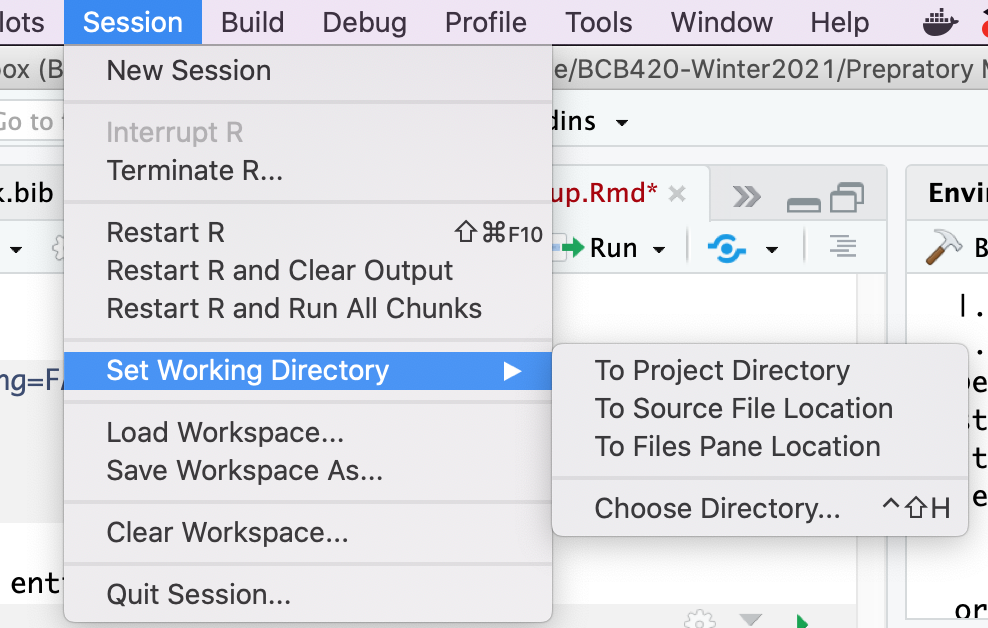
This includes the useful option to set the current project directory as the working directory 6.
Or in the Files browser in the bottom right by clicking on the More option:
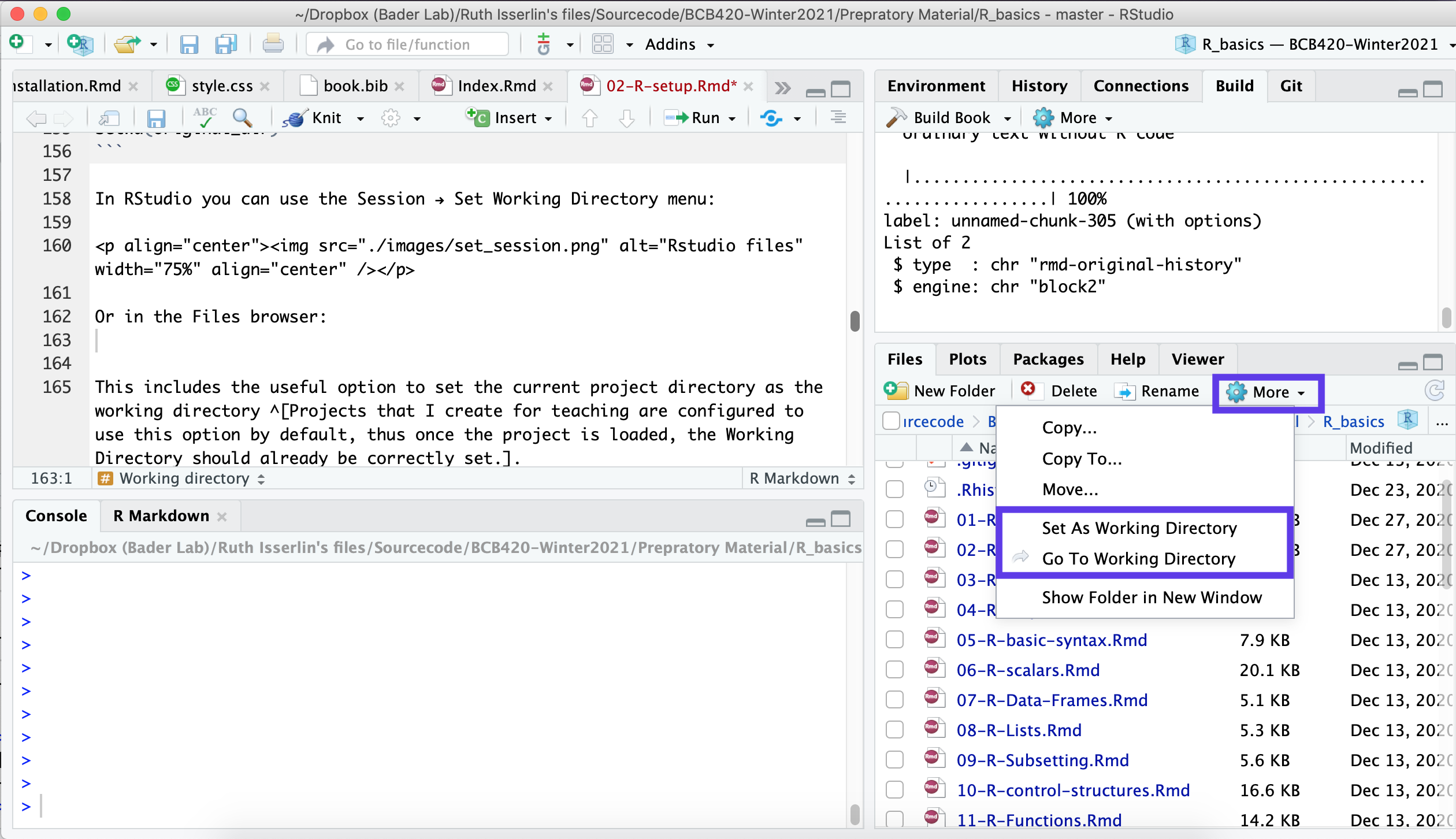
You can set the current directory to the working directory.
1.19 Task 7- Working directory
- Since you have gone through the script of the BasicSetup project, your working directory should be set to this project directory (I have configured the project to do this automatically.)
- Figure out the path to its parent directory - i.e. the course- or workshop directory you created at the beginning.
-
Use setwd(“
”) to set the Working Directory to the Course Folder. - Confirm that this has worked by typing getwd() and list.files().
- The Working Directory functions can also be accessed through the Menu, under Misc.
1.20 .Rprofile - startup commands
Often, when working on a project, you would like to start off in your working directory right away when you start up R, instead of typing the setwd() command. This is easily done in a special R-script that is executed automatically on startup7. The name of the script is .Rprofile and R expects to find it in the user’s home directory. You can edit these files with a simple text editor like Textedit (Mac), Notepad (windows) or Gedit (Linux) - or, of course, by opening it in RStudio - don’t forget that a code editor is also a text editor8.
Besides setting the working directory, other items that might go into such a file could be
- libraries that you often use
- constants that are not automatically defined
- functions that you would like to preload.
For more details, use R’s help function:
?Startup1.21 Task 8 - .Rprofile
Just for information:
- locate the .Rprofile file in the RStudio file pane;
- click on it to open it in the text-editing window.
- This way you could change it and save the changes. However, don’t do that now but Close the file again.
1.22 The “Workspace”
During an R session, you might define a large number of R-objects: variables, data structures, functions etc., and you might load packages and scripts. All of this information is stored in the so-called “Workspace”. When you quit R you have the option to save the Workspace; it will then be restored in your next session. Now, you might think: how convenient - I can just stop R, and when I restart it, it will go into the same state as it was. But no. Restoring the Workspace from a previous state is actually a bad idea: if you load data or variables in a startup script, they may be overwritten with a corrupted version that you happened to save in the workspace when you last quit. This is very hard to troubleshoot. Essentially, when you save and reload your Workspace habitually, you have overlapping and potentially conflicting behaviour of startup script and Workspace restore.
What I recommend instead is the following:
- Never save the Workspace.
- Always work from scripts.
- Write your scripts so that you can easily recreate all objects you need to continue your analysis.
- If some objects are expensive to compute, you can always save() and later load() them explicitly. In fact, restoring the Workspace does the same thing, but you have less control regarding whether the version of your objects are correct, and what temporary variables may be loaded as well.
- In this way, you work with explicit instructions, not implicit behaviour.
- Explicit beats implicit.
List the current workspace contents: initially it only contains the init() function that was loaded from the .Rprofile script on startup.
ls()## [1] "aaindex" "githistory2table" "original_dir"
## [4] "task_counter"Initialize three variables
a <- 3
b <- 4
c <- sqrt(a^2 +b^2)
ls()
## [1] "a" "aaindex" "b"
## [4] "c" "githistory2table" "original_dir"
## [7] "task_counter"Save one item in an .RData file.
save(a, file = "tmp.RData")Remove one item from the Workspace. (Note: the argument for rm() is not the string “a”, but the variable name a. No quotation marks!)
rm(a)
ls()
## [1] "aaindex" "b" "c"
## [4] "githistory2table" "original_dir" "task_counter"Load what you previously saved.
load("tmp.RData")
ls()
## [1] "a" "aaindex" "b"
## [4] "c" "githistory2table" "original_dir"
## [7] "task_counter"Note: you can save() more than one item in an .RData file. When you then load() the file, all of the objects it contains are loaded. You don’t assign these objects - they are being restored.
We can use the output of ls() as input to rm() to remove all items from the workspace. (cf. ?rm for details)
rm(list=setdiff(ls(), "task_counter"))
ls()
## [1] "task_counter"The contents of the workspace is displayed in RStudio’s Environment Pane (top-right).
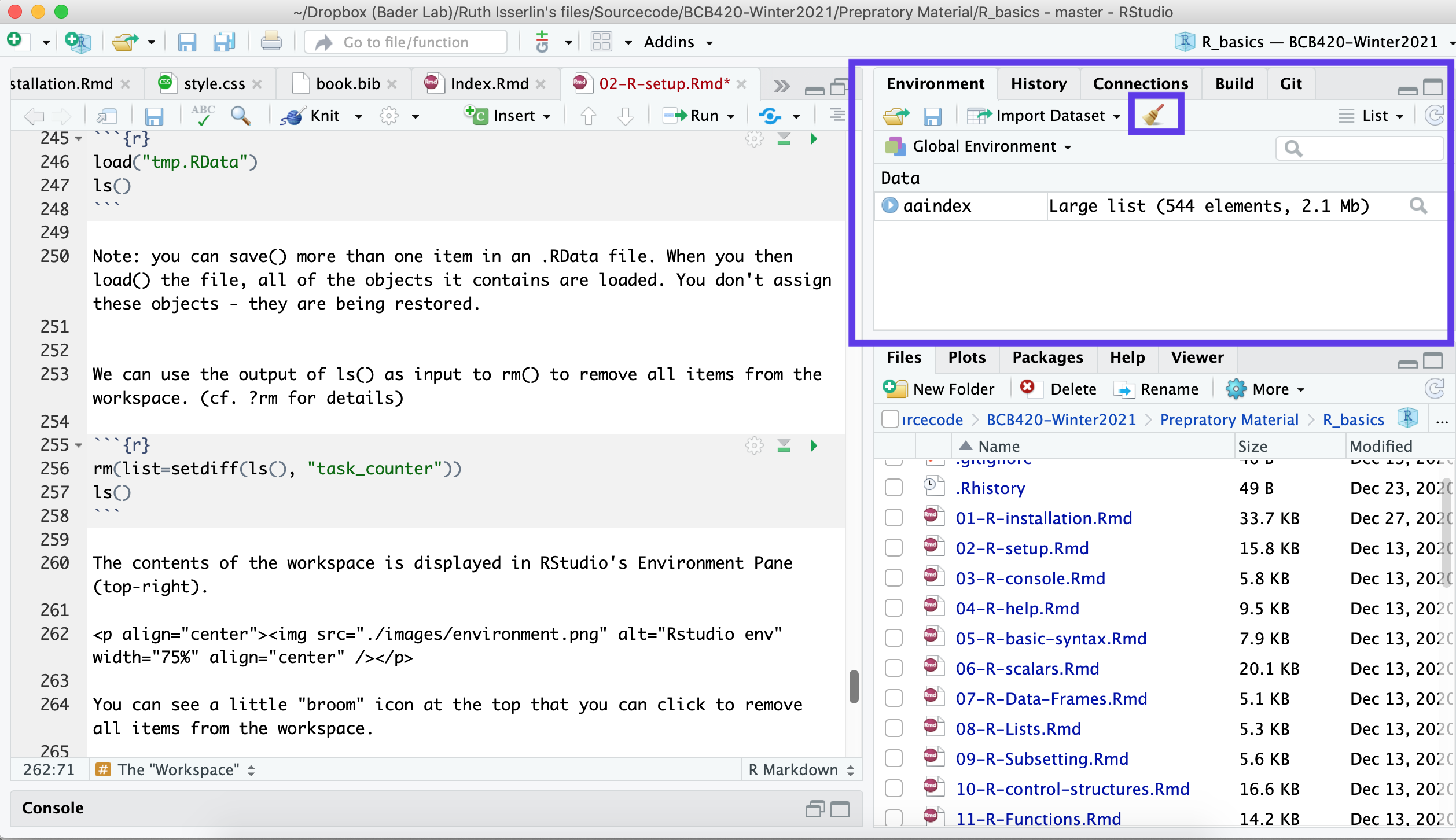
You can see a little “broom” icon at the top that you can click to remove all items from the workspace.
1.23 Self-evaluation
##Further reading, links and resources
If in doubt, ask!
If anything about this learning unit is not clear to you, do not proceed blindly but ask for clarification. Post your question on the course mailing list: others are likely to have similar problems. Or send an email to your instructor.
Author: Boris Steipe boris.steipe@utoronto.ca
Created: 2017-08-05
Modified: 2019-01-07
Version: 1.1.1
Version history:
1.1.1 Maintenance
1.1 Fixed display bug with “=” in template code; moved to GeSHi formatting.
1.0 Completed to first live version
0.1 Material collected from previous tutorial
References
and when you click on the arrow to the left, this will take you back to where you came from↩︎
Proportional fonts are for elegant document layout. Monospaced fonts are needed to properly align characters in columns. For code and sequences, we always use monospaced font.↩︎
[1] means: the following is the first (often only) element of a vector.↩︎
A “wrapper” program uses another program’s functionality in its own context. RStudio is a wrapper for R since it does not duplicate R’s functions, it runs the actual R in the background.↩︎
For example C:Documentswould be interpreted as C:Documents
ew because is the linebreak character. Even though that’s actually the path name on Windows, in an R command you have to write C:Documents/new↩︎ Projects that I create for teaching are configured to use this option by default, thus once the project is loaded, the Working Directory should already be correctly set.↩︎
Actually, the first script that runs is Rprofile.site which is found on Linux and Windows machines in the C:\Program Files\R\R-{version}\etc directory. But not on Macs.↩︎
Operating systems commonly hide files whose name starts with a period “.” from normal directory listings. All files however are displayed in RStudio’s File pane. Nevertheless, it is useful to know how to view such files by default. On Macs, you can configure the Finder to show you such “hidden files” by default. To do this: (i) Open a terminal window; (ii) Type: $defaults write com.apple.Finder AppleShowAllFiles YES (iii) Restart the Finder by accessing Force quit (under the Apple menu), selecting the Finder and clicking Relaunch. (iV) If you ever want to revert this, just do the same thing but set the default to NO instead.↩︎